OMI SO2 AMF calculations

 

1. AMF definition

 

The OMSO2 operational PBL algorithm (Krotkov et al 2006) uses differential OMTO3 residuals at 3 SO2 sensitive OMI UV2 wavelength pairs, and the pair average is used to produce slant column (SC) PBL SO2 data.

 

   (1)

 

A pre-defined Air Mass Factor (AMF) is used to estimate total SO2 (vertical column)

<

		(2)

 

Where, m(z) is vertically resolved OMI detection sensitivity to SO2 absorption (i.e. local AMF, black dashed curve in Figure 1) and n(z) is normalized SO2 vertical profile (to the unit column amount solid blue line in Figure 1).

 

Figure 1 OMI SO2 Local AMF factor (black dashed line) and normalized SO2 vertical profile (blue line)

 

Since local AMF quickly decreases with altitude, the total AMF (2) becomes a strong function of PBL SO2 profile shape. In addition AMF depends on total SO2, viewing geometry, stratospheric total ozone, surface reflectivity, and sub pixel aerosols and clouds. This makes the retrieval problem non-linear in general.

 

2. OMI SO2 public PBL AMF

 

In operational OMSO2 PBL data a constant AMF of 0.36 is used to estimate total SO2. This value represents idealized cloud and aerosol free sky conditions, slant column ozone (SCO; given by total ozone*(secSZA+secVZA)) of ~1000DU, 5% surface albedo, a typical summer PBL SO2 vertical profile (Figure 2) and 1 DU SO2 load.

 

Figure 2 SO2 quartile profiles for all summer (June-August) aircraft measurements from 2000 to 2005. [Taubman et al 2006]

 

 

With fixed SO2 profile shape (scaling approximation), spectral AMF can be calculated from the standard forward RT model (TOMRAD):

 

 

   (3)

 

where is OMI spectral airmass factor (AMF), is the N value increment due to a small column SO2 [DU] change for an aircraft SO2 profile (Table 1), g is spectral SO2 absorption coefficient convolved with OMI slit function [atm-cm] and k=100/ln(10)~43.43 is scaling constant.

 

 

Figure 3 AMF due to 1 DU in PBL for different profiles, SZA=0, NADIR, 0.05 surface albedo, 325DU mid-latitude ozone profile.

 

Figure 3 shows that spectral dependence of the AMF from the three very distinct profiles are practically identical; they differ only by a constant multiplication factor. The N-value response to the introduction to SO2 depends on both the amount of the SO2 and its vertical distribution, but one cannot separate one effect (height of SO2) from another (amount of SO2). Modeling study (Figure 3) shows that a PBL top at 800mb gives roughly the same AMF as the aircraft flights and we use that for our public release. Table 1 shows spectrally averaged AMFs assuming different PBL profiles and fixed satellite geometry (overhead sun, nadir viewing direction).

 

Table 2 Spectrally average (between 310nm and 315nm ) PBL AMF , SZA=0, nadir, Albedo =0.05

 

Top PBL SO2 profile	Average AMF	StDev AMF
500mb	0.78	0.044
700mb	0.57	0.037
800mb <2km	0.41	0.030
900 mb <1.0km	0.33	0.022
Aircraft	0.36	0.024

 

 

 

3. AMF dependence on viewing geometry (TBD)

 

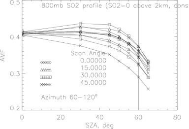
We examine AMF effect on satellite viewing geometry (Figure 4), total column ozone (Figure 5). For this analysis we will use 800mb SO2 vertical profile with all SO2 below 2km and constant mixing ration below 1.5km (Table 2).

Figure 4. 325 mid latitude ozone profile, Surf albedo 0.05

 

 

Figure 5. Same as Fig 3, but for azimuth=90deg and different TOMS ozone profiles.

 

 

Figure 6 325DU mid latitude ozone profile (dashed lines) 475DU mid-latitude profile (slid lines), azimuth 90o

 

Figure 6 shows that AMF dependence on both total ozone and viewing and solar angles can be well parameterized as function of slant column ozone:

 

   (4)

 

where W is total ozone [DU], q is nadir (scan) angle and q_o is solar zenith angle

 

Therefore OMI operational PBL data could be corrected for the actual viewing geometry and ozone as follows:

 

   (5)

 

where SO2(operational) is the OMI operational PBL SO2 values assuming constant operational AMF=0.36

 

 

4. Reflectivity dependence

 

The true AMF also depends on surface reflectivity and/or presence of aerosols/cloud. To make it easy to account for these effects we have modeled several specific cases.

 

 

Figure 7. AMF dependence on surface albedo

 

Figure 7 shows AMF dependence on surface reflectivity. Two regression curves are provided for surface albedos 0.05 and 0.1. User can first interpolate regression coefficients to obtain a single regression curve for specific albedo and then use interpolated regression with equation (5) to correct OMI operational So2 data.

 

 

 

4. Aerosol corrections

 

In a similar approach, specific AMF correction can be developed to correct for aerosol effects. The main aerosol parameters affecting AMF are : vertical distribution, aerosol optical thicknedd (AOT) and Single scattering albedo (SSA) at 310nm. Figure 8 shows effect of AOT and figure 9 shows effect of SSA both assuming similar aerosol vertical distributions.

 

Figure 8. AMF dependence on aerosol AOT

 

Figure 8 shows that weakly absorbing aerosol (sulfate) considerably enhances AMF with some saturation at AOT₅₀₀> 0.5 (AOT₃₀₀> 1.0 ). We should note that AOT at 310nm is roughly twice the AOT at 500nm for pollution aerosol models (small particles, Angstrom parameter >1 ). On the other hand, increasing aerosol absorption (SSA drops from 0.97 to 0.9) decreases AMF (Figure 8). So the two aerosol effects move AMF in opposite directions: aerosol scattering enhances AMF and aerosol absorption reduces it.

Figure 9. AMF dependence on single scattering albedo

 

This could be further illustrated comparing effects of pollution and dust aerosols on OMI SO2 measurements over China. As can be seen from the figure dust aerosols considerably reduce AMF while weakly absorbing pollution aerosols have a minimal effect (due to cancellation of scattering and absorption effects).

Figure 10. AMF dependence on 2 aerosol models

 

 

 

 

5. Cloud corrections

 

The effect of clouds is not considered in current version. The assumption is that clouds always screen PBL SO2, but no AMF correction is attempted to account for this invisible SO2. This cloud related AMF error becomes larger with increasing sub-pixel cloudiness, so that fill values are used if OMTO3 cloud fraction is larger than ~20%, which corresponds to LER ~30%.